The Setup

In this tutorial, we will learn how to make smooth transitions between animated objects. This can be e.g. useful for camera rigging, as you can see in this video:

Let’s start with a simple scene: We have a slow moving blue torus, and a fast moving red torus, both with constant velocity.

We now want to add a purple pin needle that smoothly transitions from object to the next one.

You can either follow this tutorial step by step, or download the ready-made Blender file here (created with Blender 5.1). Download Scene 1 (.blend)

Linear Interpolation (Lerp)

Now, we add a purple pin needle, which will first start from the blue cylinder, and will translate to the red one. This can be done with a simple mix node.

This already works great!

Speaking in terms of math, we have a lerp function here.

$$\textcolor{purple}{\operatorname{lerp}}(\textcolor{blue}{a}, \textcolor{red}{b}, \textcolor{green}{t}) = \textcolor{blue}{a} + (\textcolor{red}{b} - \textcolor{blue}{a}) \cdot \textcolor{green}{t}$$

Where:

• $\textcolor{purple}{\operatorname{lerp}}(\textcolor{blue}{a}, \textcolor{red}{b}, \textcolor{green}{t})$ is the position of the purple needle
• $\textcolor{blue}{a}$ is the position of the blue torus
• $\textcolor{red}{b}$ is the position of the red torus
• $\textcolor{green}{t}$ is the mix factor, where $\textcolor{green}{t} = 0$ means completely on the blue side, and $\textcolor{green}{t} = 1$ means completely on the red side

Recursive Lerp for Extra Smoothness

Can we get the transition even smoother? Yep! Now we add a new, this time orange pin needle, that is “pulled” by the purple one.

And guess what, the position of the orange pin is as well calculated by a lerp function. But this time a bit different. It’s a recursive lerp function with a constant t factor. The t factor is at 0.1, which means “with every frame that passes, move the orange needle 10% closer to the purple needle”.

Here’s the formula:

$$\textcolor{#CC7000}{x_{n+1}} = \operatorname{lerp}(\textcolor{#CC7000}{x_n}, \textcolor{purple}{p_n}, \textcolor{green}{t}) = \textcolor{#CC7000}{x_n} + (\textcolor{purple}{p_n} - \textcolor{#CC7000}{x_n}) \cdot \textcolor{green}{t}$$

Where:

• $\textcolor{#CC7000}{x_n}$ is the current position of the orange needle at frame $n$
• $\textcolor{#CC7000}{x_{n+1}}$ is the position of the orange needle at the next frame
• $\textcolor{purple}{p_n}$ is the current position of the purple needle (itself the lerp between blue and red)
• $\textcolor{green}{t} = 0.1$ is the constant smoothing factor. Each frame, the orange needle closes 10% of the remaining gap to the purple needle

Notice the key difference to the lerp from the last chapter: the formula depends on its own previous result ($\textcolor{#CC7000}{x_n}$). This is why we need a Simulation Zone in Geometry Nodes. Regular Geometry Nodes are stateless: They compute everything from scratch each frame with no memory of previous frames. But our recursive lerp needs to remember where the orange needle was last frame to compute where it should be next. The Simulation Zone gives us exactly that: it carries state across frames, feeding $\textcolor{#CC7000}{x_{n+1}}$ back in as $\textcolor{#CC7000}{x_n}$ on the next frame.

Compensating for Lag with Velocity

There’s a problem though: the orange needle is always lagging behind the purple one. Because it only ever closes a fraction of the gap each frame, it can never truly catch up.

To fix this, we can give each needle a little push forward by adding a velocity term. Instead of lerping toward the current position of the target, we lerp toward a predicted position: the target’s current position plus its speed scaled by some factor.

The upside-down pins show where each torus will be in the near future. By using the predicted positions, we have now a better positioning of the orange pin.

Attaching a Camera

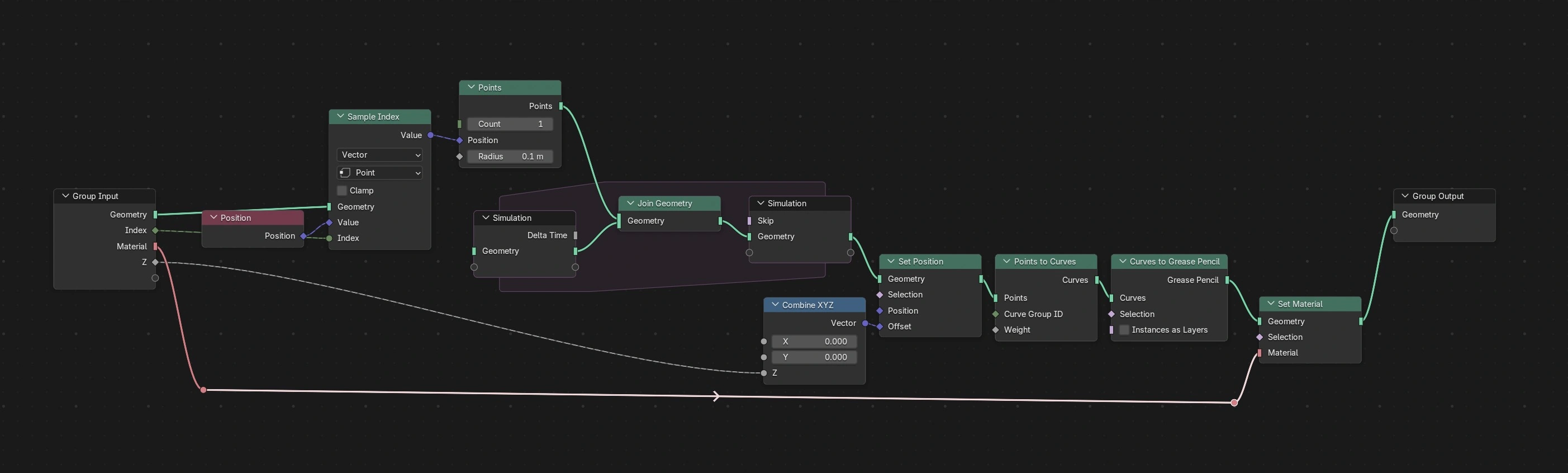
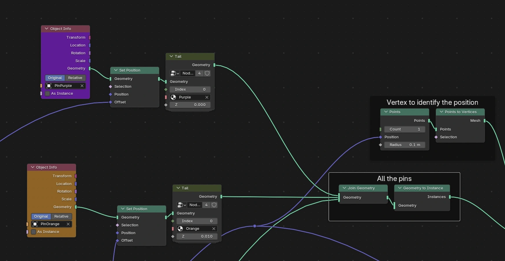
Now that the orange needle follows a nice smooth path, we can use it to drive a camera. The first step is to create a vertex at the position of the orange pin. This gives us a point in space that Blender’s camera constraints can track.

We do this by adding a Points node (count = 1), feeding the orange pin’s location into it, and converting it to a mesh vertex with Points to Vertices. This vertex is then joined into the output geometry.

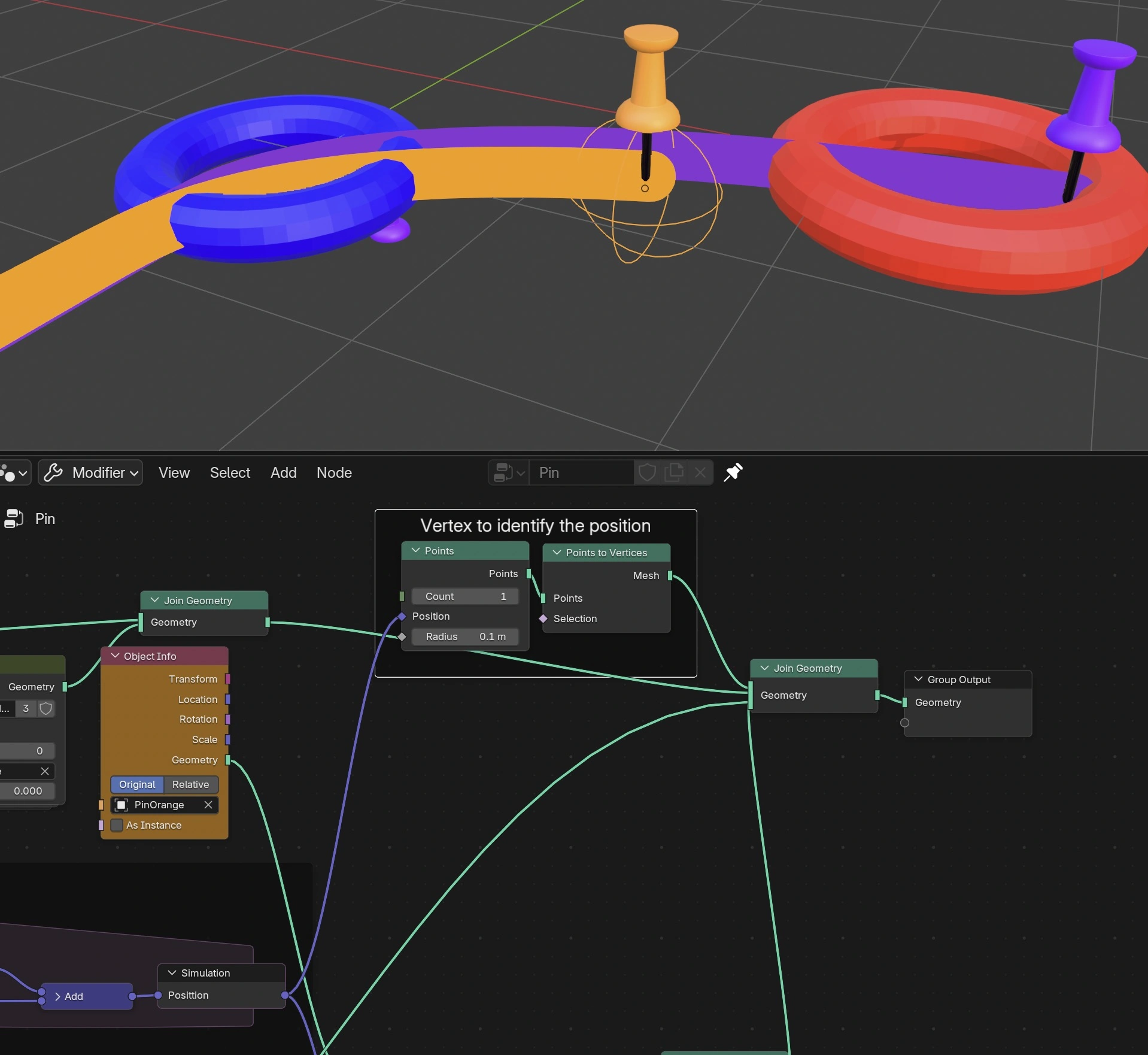
Note that the single vertex must come first in the Join Geometry node.

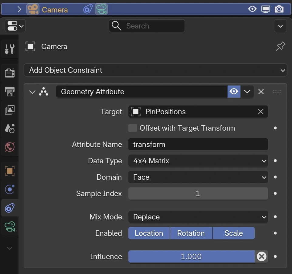
Next, we add an Empty and assign it a “Geometry Attribute” constraint. This constraint reads the position attribute from the vertex we just created, so the Empty automatically follows the orange pin’s position every frame. Set the Sample Index to 0.

And here we go, the final scene is ready!

Download Scene 1 (.blend) — same file as above

What’s Next: Moving the Camera in 3D Space

With this setup, we only track the Empty with a “Track To” constraint on the camera. The camera always looks at the orange Pin, but it stays fixed in place. Wouldn’t it be cool if the camera itself could also move through 3D space, following the object, fully controlled from Geometry Nodes?

That’s also possible with the “Geometry Attribute” constraint, let’s take a closer look!

Download Scene 2 (.blend)

Now, let’s take a look from the top.

We see the camera tail is moving exactly the same as the orange pin. That’s great! But we can also see two extra planes that were added.

So here’s how this works. These planes are controlled by the position of the orange pin. We use this Geometry Nodes setup:

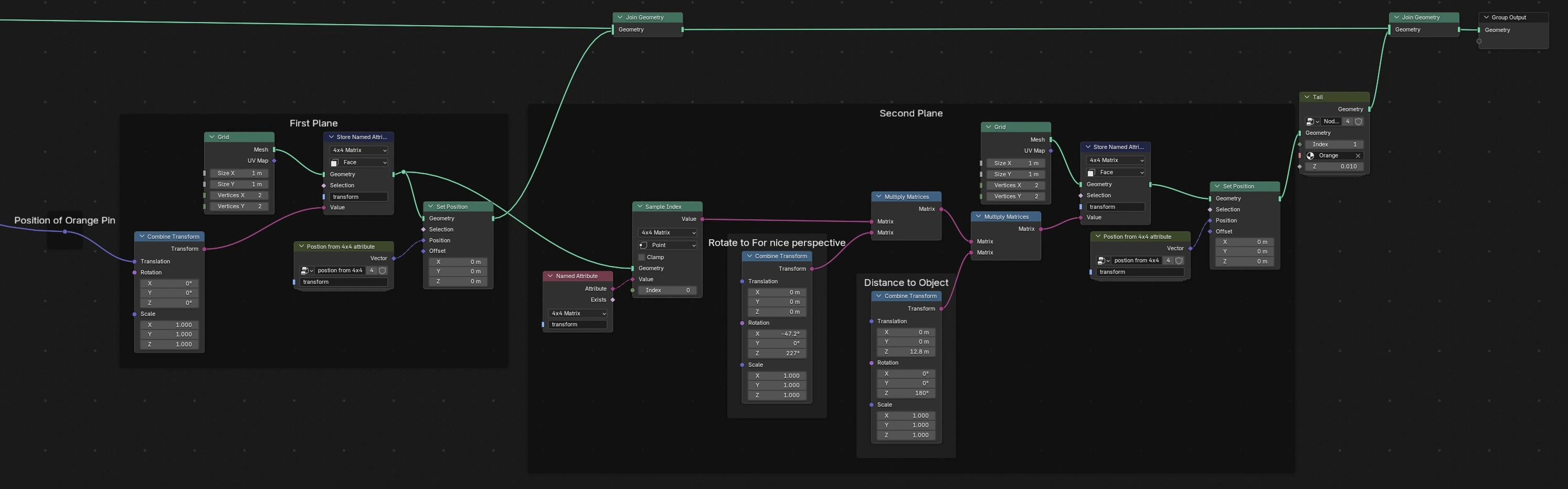
Note that we save a 4x4 matrix (contains position, rotation and scale) in the faces of these planes. That’s great because we can later use them in a “Geometry Attribute” constraint on the camera:

Also here the order how the geometry is joined matters. It’s a good idea to have a look at the spreadsheet to see where this matrix is stored:

In order to not clutter the spreadsheet too much, we can first put all pins into a “Geometry to Instance” node, so that we don’t have to scroll through hundreds of columns.

Now we have everything in place.

Download Scene 2 (.blend) — same file as above

Ideas to Explore Further

This setup is a solid foundation, and there’s a lot you can build on top of it:

• Random noise for handheld camera shake
• Camera roll and tilt driven by the velocity direction
• Slerp (spherical linear interpolation) for smoother rotational blending between targets